Staff Removal in PyTorch (Revisiting ICDAR 2013)

2012 was a significant year for computer vision, as AlexNet smashed past records (and same-year competitors) on the ImageNet recognition challenge. In the following months and years, the field embraced CNN-based techniques, and a vast number of tasks and benchmarks saw major improvements in performance. Because of this, and thanks to the maturity of modern deep learning frameworks, it is quite often the case that pre-deep-learning challenges and benchmarks can be trivially surpassed, often with huge margins, simply by using basic out-of-the-box deep learning techniques.

ICDAR Challenge

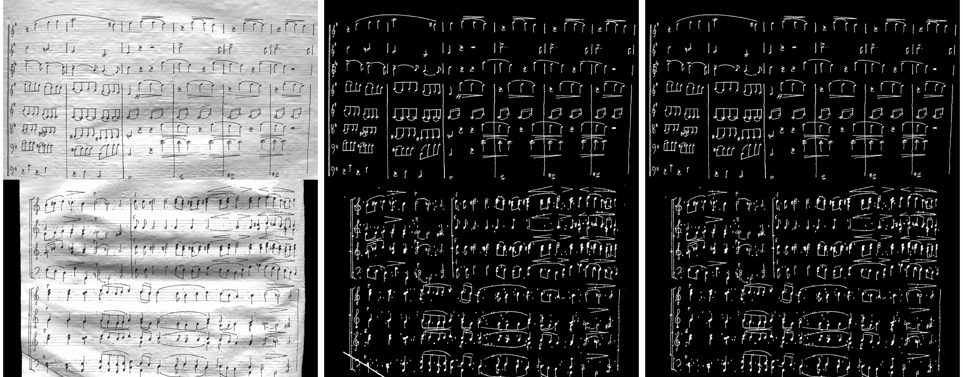
Hosted in 2013, the goal of this challenge was to take as input images of sheet music (either binary or grayscale), and then output a binary mask of the sheet music elements, but without the staff lines. Here are some examples (grayscale input, binary input, target result):

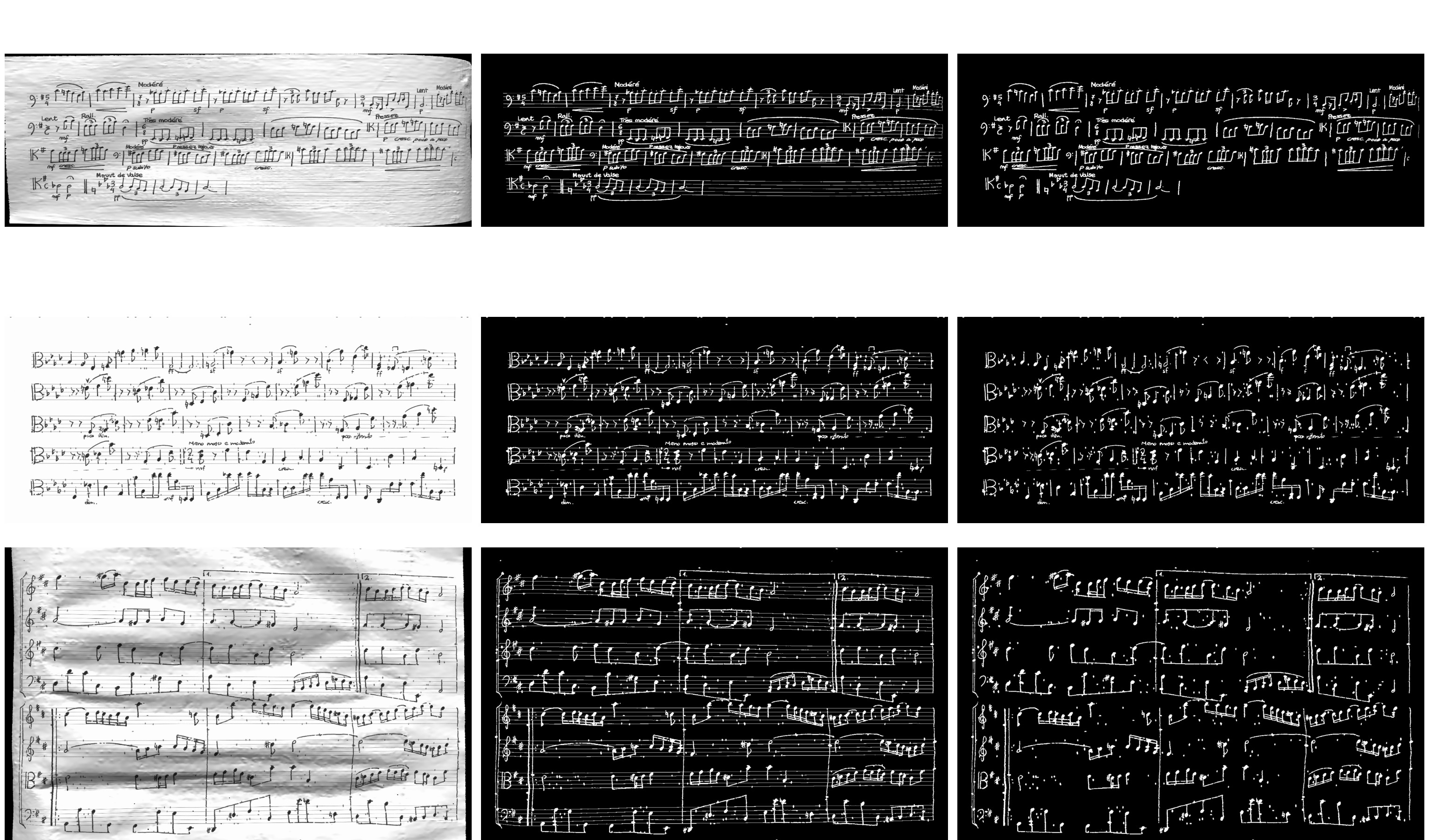
Using grayscale input is clearly a harder problem, given the increased domain and noise. Both types of input are also subject to a variety of noise and geometric distortions, and the handwritten nature of the scores increases variance among samples.

The training set (and test set) are divided into sections, with each section having varying amounts of degradation (noise and distortion) applied to it, to provide different levels of difficulty on which to evaluate submitted results. See the website and published results for more details.

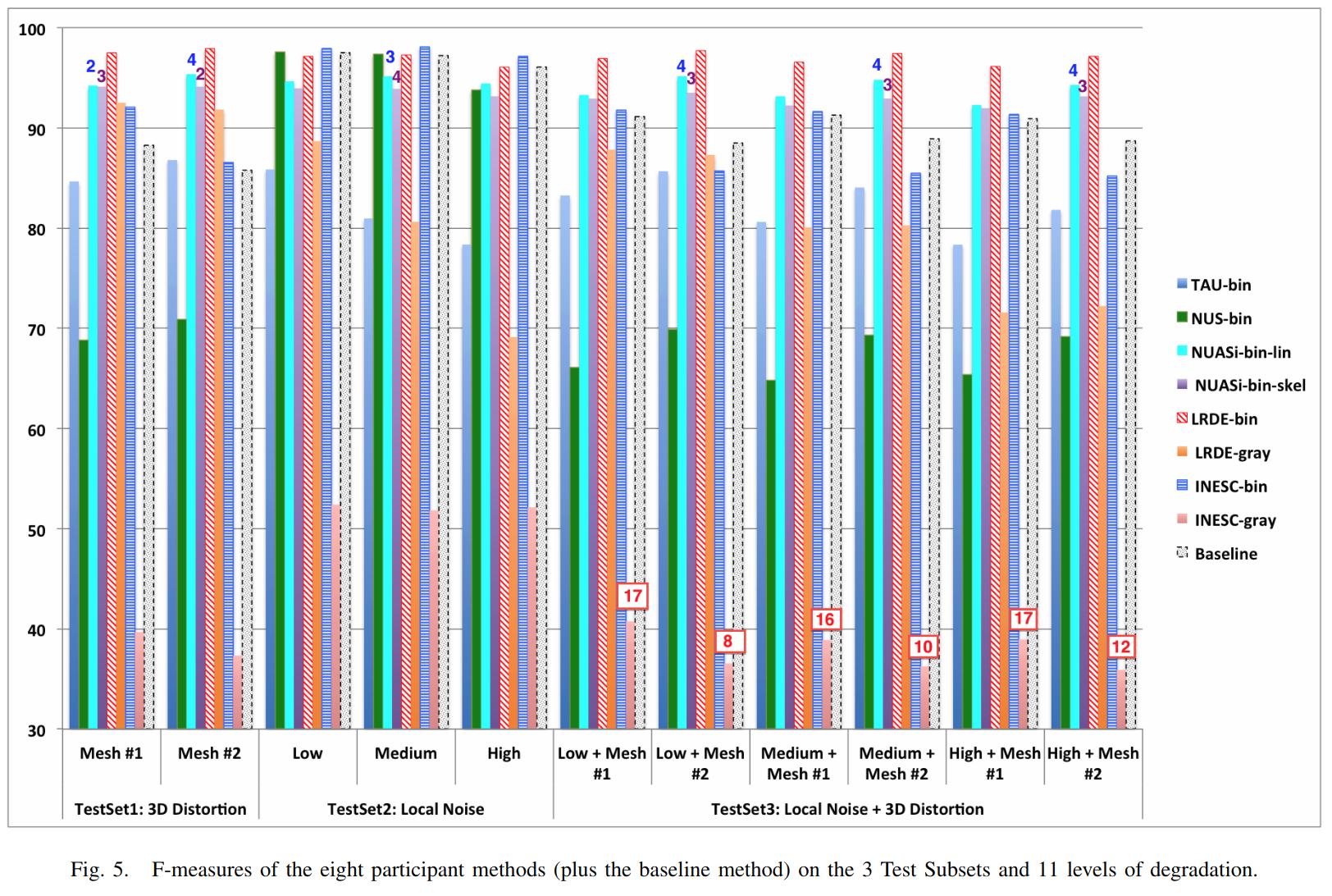
From the published results, we see that a variety of heuristics-based techniques were submitted. The top performers have very good F1-scores given binary input, or with low amounts of degradation, but results on grayscale images with higher degradation are not as good, with the best F1-scores a little over 70.

As an aside, you may be wondering why staff removal is a useful task at all. In the pre-deep-learning era, many OMR (optical music recognition) systems were built as pipelines of sequential heuristic-based algorithms. Cleaning up the staff as a preprocessing step was useful to simplify downstream steps. Now that end-to-end learning has become more powerful, staff removal as a discrete step will likely fall out of favor (though staves will probably continue to be identified as part of more general segmentation tasks).

Preparing Training Data

Given the unfair advantage of 7 years of deep learning advancement, we’re obviously going to try the solve the hardest challenge, with grayscale input and the maximum amount of noise and distortion. After downloading the training data from the website, we’ll need to write a data loader class, to load in images and convert them to appropriate tensors.

Because the images are fairly high-resolution, using them directly is not feasible, at least not with my limited amount of GPU memory. We thus have 2 choices: either downsample the images, or operate on patches of images. Zooming in, we can see that some staff lines are only 1 pixel wide, so downsampling could lose some important data.

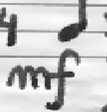
Also, identifying staff lines shouldn’t require much spatial context - given this 512x512 patch, it’s easy to see which pixels correspond to staff lines. In fact, we could likely go much lower than 512x512, though I have not tried.

We’ll set up our data pipeline to extract patches from images, and classification will be performed one patch at a time. Here’s what the data loader code looks like. Note the slightly awkward usage of RandomCrop’s parameters passed to functional crop methods. Apparently this is somewhat by design/the recommended way.

class StaffImageDataset(Dataset):
    def __init__(self, in_files, gt_files, size=(512, 512)):
        self.in_files = in_files
        self.gt_files = gt_files
        self.size = size

    def __getitem__(self, index):
        in_image = Image.open(self.in_files[index])
        gt_image = Image.open(self.gt_files[index])

        y, x, h, w = transforms.RandomCrop.get_params(in_image, output_size=self.size)

        in_image = TF.crop(in_image, y, x, h, w)
        gt_image = TF.crop(gt_image, y, x, h, w)
        return (TF.to_tensor(in_image), TF.to_tensor(gt_image))

    def __len__(self):
        return len(self.in_files)

It’s a little inefficient to load in a large image just to use one small patch - we risk bottlenecking by disk IO, and could instead extract multiple patches at a time. However, I found running DataLoaders in parallel kept my GPU utilization maximized.

in_train, in_test, gt_train, gt_test = train_test_split(in_files, gt_files, test_size=0.1, random_state=0)
train_dataset = StaffImageDataset(in_train, gt_train)
test_dataset = StaffImageDataset(in_test, gt_test)
train_data_loader = DataLoader(train_dataset, batch_size=batch_size, shuffle=True, num_workers=data_loader_parallel)
test_data_loader = DataLoader(test_dataset, batch_size=batch_size, shuffle=True, num_workers=data_loader_parallel)

Network Choice

The class of problem we are looking to solve is semantic segmentation, in which every pixel is assigned a label. This a very broadly studied area, with thousands of papers and network architectures. We’ll use UNet, which is one of the earlier and simpler architectures, from 2015.

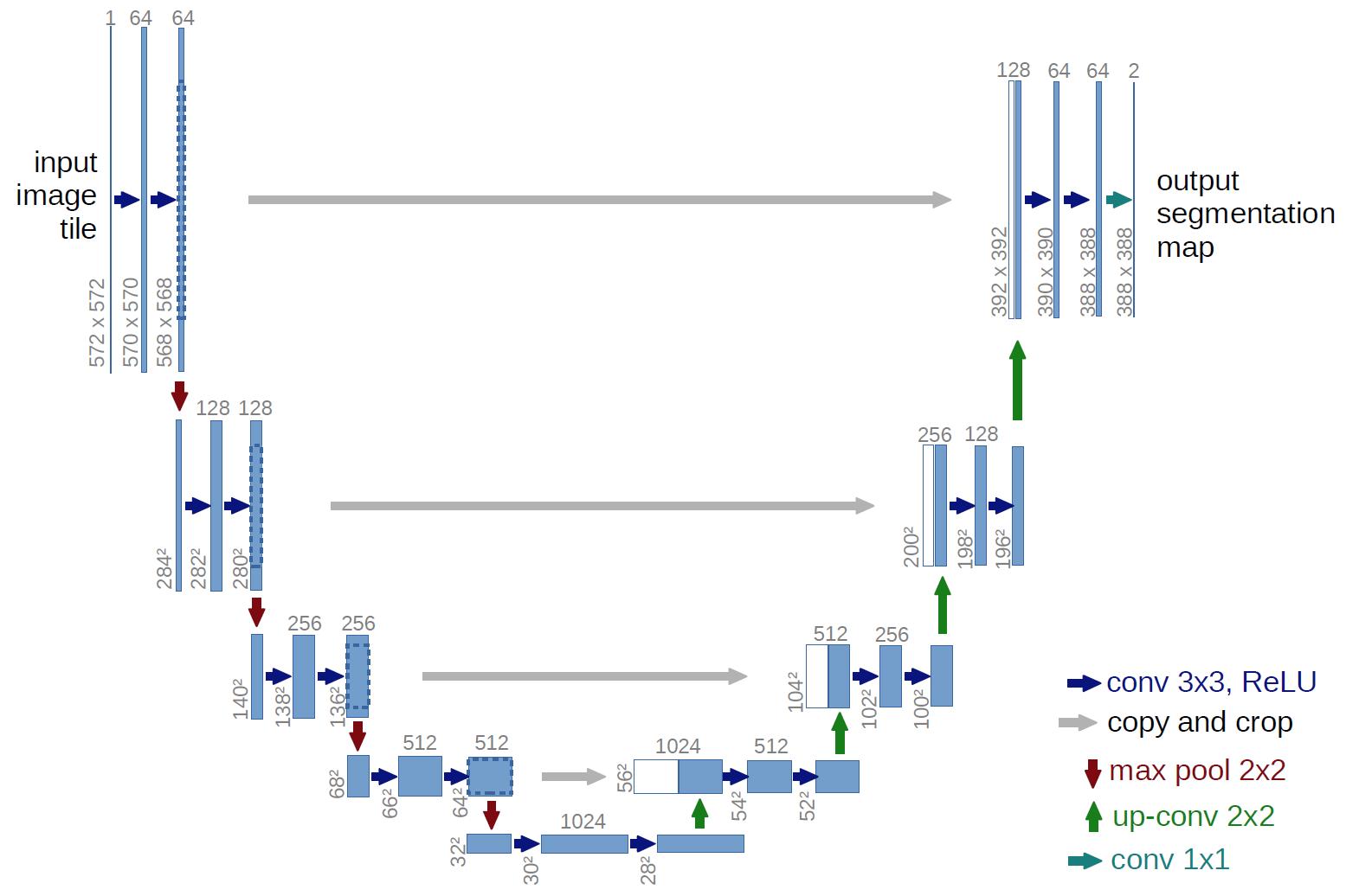
The basic idea, which is now extremely common, is to have a series of contraction layers followed by a series of expansion layers. The contraction layers accumulate spatial information into higher-level features, while the expansion layers spread that higher-level understanding back across pixels. Skip connections are used to preserve high-resolution detail across intermediate levels. Although there are many fantastic open-source implementations available, I decided to implement it myself, just to practice with pytorch and show how easy it is to build up these simpler network architectures.

import torch
from torch import nn

# UNet is composed of blocks which consist of 2 conv2ds and ReLUs
def convBlock(in_channels, out_channels, padding):
    return nn.Sequential(
        nn.Conv2d(in_channels, out_channels, 3, padding=padding),
        nn.ReLU(),
        nn.Conv2d(out_channels, out_channels, 3, padding=padding),
        nn.ReLU()
    )

# Skip connections are concatenated, cropping if size changed due to no padding
def cropAndConcat(a, b):
    if (a.shape == b.shape):
        return torch.cat([a, b], 1)

    margin2 = (a.shape[2] - b.shape[2]) // 2
    margin3 = (a.shape[3] - b.shape[3]) // 2
    a_cropped = a[:, :, margin2 : margin2 + b.shape[2], margin3 : margin3 + b.shape[3]]
    return torch.cat([a_cropped, b], 1)

class UNet(nn.Module):

    # Depth includes the bottleneck block. So total number of blocks is depth * 2 - 1
    # Unexpected output sizes or num channels can occur if parameters aren't nice
    # powers of 2
    def __init__(self,
                 input_channels=1,
                 output_channels=2,
                 depth=5,
                 num_initial_channels=64,
                 conv_padding=0
                 ):
        super().__init__()

        # Going down, each conv block doubles in number of feature channels
        self.down_convs = nn.ModuleList()
        in_channels = input_channels
        out_channels = num_initial_channels
        for _ in range(depth-1):
            self.down_convs.append(convBlock(in_channels, out_channels, conv_padding))
            in_channels = out_channels
            out_channels *= 2

        self.bottleneck = convBlock(in_channels, out_channels, conv_padding)

        # On the way back up, feature channels decreases.
        # We also have transpose convolutions for upsampling
        self.up_convs = nn.ModuleList()
        self.tp_convs = nn.ModuleList()
        in_channels = out_channels
        out_channels = in_channels // 2
        for _ in range(depth-1):
            self.up_convs.append(convBlock(in_channels, out_channels, conv_padding))
            self.tp_convs.append(nn.ConvTranspose2d(in_channels, out_channels,
                                                    kernel_size=2, stride=2))
            in_channels = out_channels
            out_channels //= 2

        # final layer is 1x1 convolution, don't need padding here
        self.final_conv = nn.Conv2d(in_channels, output_channels, 1)

        # max pooling gets applied in a couple places. It has no
        # trainable parameters, so we just make one module and reuse it.
        self.max_pool = nn.MaxPool2d(2)

    def forward(self, x):
        features = []
        for down_conv in self.down_convs:
            features.append(down_conv(x))
            x = self.max_pool(features[-1])

        x = self.bottleneck(x)

        for up_conv, tp_conv, feature in zip(self.up_convs, self.tp_convs, reversed(features)):
            x = up_conv(cropAndConcat(feature, tp_conv(x)))

        return self.final_conv(x)

The 3 main parameter choices are number of layers, initial number of feature channels, and type of padding. I initially tried 5 layers, 64 features, valid padding, as is used in the paper. The number of parameters took up a lot of my gpu memory though, and training was quite slow. I switched to 3 layers and 32 features, which drastically reduced memory usage and sped up training time. It’s likely network size could be reduced more without much effect on performance (after all UNet has been used to solve much harder problems than this), but I did not test further. I also switched from valid padding to zero padding, which means border pixels are influenced by “fake” values. This is often argued to perform worse, but it makes the data handling a bit simpler, as output sizes match input sizes.

Training

With a data loader and a network, all that’s left is to train. We simply pick an optimizer and loss function (both just arbitrary default-ish choices), and put together a basic training loop. I use apex.amp to support larger batch sizes on my local GPU.

epochs=10
learning_rate=0.001

device = torch.device('cuda:0' if torch.cuda.is_available() else 'cpu')
net = UNet(depth=3, num_initial_channels=32, conv_padding=1).to(device)

criterion = torch.nn.CrossEntropyLoss()
optimizer = torch.optim.Adam(net.parameters(), lr=learning_rate)

net, optimizer = amp.initialize(net, optimizer, opt_level="O1")

# The training loop
total_steps = len(train_data_loader)
for epoch in range(epochs):
    net.train()
    for i, (in_images, gt_images) in enumerate(train_data_loader, 1):
        preds = net(in_images.to(device))
        gt_images = gt_images.squeeze(1).type(torch.LongTensor).to(device)
        loss = criterion(preds, gt_images)

        optimizer.zero_grad()
        with amp.scale_loss(loss, optimizer) as scaled_loss:
            scaled_loss.backward()
        optimizer.step()

        if (i) % 10 == 0:
            print (f"Epoch [{epoch + 1}/{epochs}], Step [{i}/{total_steps}], Loss: {loss.item():4f}")

    # Save after each epoch
    torch.save({'epoch': epoch,
                'model_state_dict': net.state_dict(),
                'optimizer_state_dict': optimizer.state_dict(),
                'loss': loss
    }, 'checkpoint' + str(epoch) + '.ckpt')

    # Evaluate validation after each epoch
    net.eval()
    with torch.no_grad():
        sum_loss = 0
        for in_images, gt_images in test_data_loader:
            preds = net(in_images.to(device))
            gt_images = gt_images.squeeze(1).type(torch.LongTensor).to(device)
            sum_loss += criterion(preds, gt_images)
        print(f'validation loss: {(sum_loss / len(test_data_loader)):4f}')

Results

With this basic network and training setup, each epoch took around 2 minutes to train for me, and validation loss flattened out after 5 epochs, for a total training time of 10 minutes. Note that these training images are around 8 megapixels, and I only sampled 512x512 patches from them. That means my overall training run only looked at around 15% of available pixels before saturating.

With our binary-patch-semantic-segmentation network trained, we can now classify each patch in each image in the test set. Note that we would likely get best results by overlapping patches and combining their predictions, but I simply used adjacent patches, overlapping as needed at the borders to fit irregular image dimensions.

Here are 2 inputs, followed by predictions and ground truths, where the first case is an “easy” sample, and the second has more noise. Interestingly, point noise as visible in the bottom sample is kept in the ground truth output, and our network learned to do the same. Our network is fooled by the crease in the lower-left corner though.

After running inference on the test set, we can compute our score using the test ground truth published after the competition. Recall that the top submissions in 2013 reached an F1 score around 0.72. With our basic UNet and 10 minutes of training, we obtain an F1 score of 0.966 across all 2000 test images. Looking at just the 1000 test images with the highest levels of degradation, F1 score only drops to 0.959.

This is really no surprise considering the much more complex problems being tackled these days, but it’s nice to look at what can be solved with just the bare minimum of today’s techniques.